Le rapport sur l’état de l’environnement 2022 est un document technique destiné à un usage interne. Il n’est disponible qu’en anglais.

Introduction 

This section deals with global phenomena that influence human activities and the environment. Relevant environmental topics, called focal points, look at changes in global climate and environmental trends, greenhouse gas emissions, and world population.

This group of indicators tracks important global driving forces that influence long-term changes at the global scale. They provide information used in other focal points to analyze why some indicators are changing in the NWT. These changes can have significant direct and indirect effects on the NWT environment. They set the stage for more detailed NWT indicators across other critical areas of focus.

1.1 Trends in global population numbers

This indicator reports on past, present, and future projected changes in human populations on our planet.

NWT Focus

The increasing global human population is linked directly and indirectly to increases in greenhouse gas emissions, changes in long-range contaminants, and changes in the demand for resources from the NWT.

In the long term, Canada and the NWT may notice direct impacts as the combination of a growing global human population and the increasing effects of climate change leads to a rise in climate refugees migrating away from areas experiencing extreme impacts as a result of these changes. An estimated 23.9 million people were displaced by weather-related disasters in 2019 alone. This is the greatest number recorded since 2012. These disasters include floods, hurricanes, wildfires, droughts, and extreme temperatures (Ref. 1).

Projections for future numbers of climate refugees are wide-ranging because they are dependent upon several environmental, socioeconomic, and political factors that are difficult to predict. However, it is estimated that up to 200 million people could be affected by climate impacts and become climate refugees by 2050 (Ref. 2, 3). It has been noted that the number of refugee applications in the European Union correlates to temperature fluctuations. These applications are forecasted to rise by 188% (660,000) per year by the end of the century under a high emissions scenario (Ref. 4).

Due to the recent ruling by the UN Human Rights Committee (Ref. 5) which found nations are obliged to not forcibly return individuals to locations where climate change poses a threat to their right life, Canada, like all nations, is required to consider climate change as legitimate grounds for refugee status.

Current View: status and trend

This indicator is informed by past, pesent and future trends. Figure 1 below shows best estimates of the global human population from 10,000 BCE to present day and projections forward to 2050. This graph illustrates the exponential population growth that has occurred over just the last two centuries.

Figure 1: Historical World Population Since 10,000 Before Common Era. Adapted with permission from “One Small Planet, Seven Billion People by Year’s End and 10.1 Billion by Century’s End” (Ref. 6), with updated data from United Nations Population Division (2018) (Ref. 7).  Reproduced with permission from the United Nations Environment Programme.

The estimated population of the world reached 7.7 billon people in 2019 (Ref. 8). However, the overall rate of population growth has been slowing since the 1960s due to a reduction in birth rates. Population growth ranges peaked at 2.1% in 1965-1970, and they are currently below 1.1% in 2021 (Ref. 8). Currently, the growth rate continues to decline, which can be observed in Figure 2.

Figure 2: Global Population Size and Annual Growth Rate Projection (1950 – 2100). From “World Population Prospects 2019 Highlights” (Ref. 8).  Reproduced with permission through a United Nations Creative Commons license.

 

Looking forward

Projecting future global human population growth is difficult. It depends on many factors, including world events, fertility policies, and disease prevention programs. The United Nations uses all available sources of data on population size, levels of fertility, mortality, and international migration when projecting future populations globally and within each region of the world (Ref. 8). The United Nations predicts global human population to reach 9.7 billion in 2050, and that it will peak at around 10.9 billion by 2100 (Ref. 8). See Figure 2 for an estimated projection of world population growth.

Figure 3: Global Population Size and Annual Growth Rate Projection (1950 – 2100), broken down by region. Reproduced with permission from “World Population Prospects 2019 Highlights” (Ref. 8) through a United Nations Creative Commons license. The projections depict confidence intervals through shading that increase further into the future.

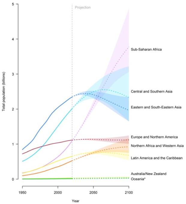
While global population growth is a useful indicator of the overall picture of changing world populations, it is also useful to review population growth by region, as each region differs. Figure 3 shows past and future population growth by region. As seen in the graph, Asia is currently the most populous region of the world by far. However, almost every region in the world is projected to peak in population in the very near future, followed by a decline or flatline. This projected peak and decline is driven by falling fertility rates in every region of the world. The exception is Africa, in particular sub-Saharan Africa, which is projected to have significant population growth for the remainder of the century, with the population not peaking prior to 2100. In fact, most of the projected global population growth to 2100 will be driven by sub-Saharan Africa.

While sub-Saharan Africa is experiencing a reduction in fertility much like the rest of the world, they still have the highest fertility rate in the world (4.6 live births per woman in 2019), and it is not projected to reduce substantially enough to significantly slow or stop their high population growth before 2100. By 2050, their fertility rate is projected to be 3.1 live births per woman, which is still significantly above replacement level and still greater than the projected fertility rate of any other region on earth (Ref. 8).

Migration also affects population growth of various regions. In areas experiencing negative natural population growth, such as parts of Europe, immigration lessens the effects of decreasing population size.

 

Technical Notes

The United Nations Department of Economic and Social Affairs (UNDESA) compiles, generates and analyses a wide range of economic, social and environmental data. The Population Division of the UNDESA “provides the international community with timely and accessible population data and analysis of population trends and development outcomes for all countries and areas of the world” (Ref. 8). The Division regularly undertakes studies of population size and characteristics of fertility, mortality and migration. They provide “substantive support on population and development issues to the United Nations General Assembly, the Economic and Social Council, and the Commission on Population and Development” (Ref. 8).

The World Population Prospects 2019: Highlights paper provides a summary of the twenty-sixth edition of official United Nations population estimates and projections. It presents population estimates for 235 countries or areas, along with analyses of historical demographic trends. The assessment “considers the results of 1,690 national population censuses conducted between 1950 and 2018, as well as information from vital registration systems and from 2,700 nationally representative sample surveys.” The assessment also “presents population projections to the year 2100 that reflect a range of plausible outcomes at the global, regional and country levels.” (Ref. 8).

 

References

Ref. 1.  Internal Displacement Monitoring Centre. 2020. “Global Report on Internal Displacement 2020”.

Ref. 2.  Myers, Norman. 2002. Environmental refugees: a growing phenomenon of the 21st century. Phil. Trans. R. Soc. Lond. B (2002) v. 357, pp. 609-613.

Ref. 3.  International Federation of Red Cross and Red Crescent Societies. 2019. “The Cost of Doing Nothing: The Humanitarian Price of Climate Change and How it Can Be Avoided”. Geneva, 2019.

Ref. 4.  Missirian A, Schlenker W. 2017. Asylum applications respond to temperature fluctuations. Science. 2017 Dec 22;358(6370):1610-1614. Available at: doi: 10.1126/science.aao0432.

Ref. 5.  Sinclair-Blakemore, Adaena. 2020. “Teitiota v New Zealand: A Step Forward in the Protection of Climate Refugees under International Human Rights Law?” (OxHRH Blog, 2020) Available at: http://ohrh.law.ox.ac.uk/teitiota-v-new-zealand-a-step-forward-in-the-protection-of-climate-refugees-under-international-human-rights-law [accessed May 21, 2021]

Ref. 6.  United Nations Environment Programme – Global Environmental Alert Service. 2011. “One Small Planet, Seven Billion People by Year’s End and 10.1 Billion by Century’s End”. Available at: https://na.unep.net/geas/getuneppagewitharticleidscript.php?article_id=71.

Ref. 7.  United Nations, Department of Economic and Social Affairs, Population Division. 2018. World Urbanization Prospects: The 2018 Revision, custom data acquired via website.

Ref. 8.  United Nations, Department of Economic and Social Affairs, Population Division. 2019. World Population Prospects 2019: Highlights.

 

1.2 Trends in average temperature, ocean heat content, snow cover, ocean levels, precipitation and acidity

This indicator reports on measured changes in global temperature and ocean changes.

This indicator was prepared by the Government of the Northwest Territories, Department of Environment and Climate Change, with information summarized primarily from the Fifth Assessment Report of the Intergovernmental Panel on Climate Change (IPCC), the 2019 IPCC Special Report, and the National Oceanic and Atmospheric Administration (NOAA).

 

NWT Focus

Increases in temperature, and changes in oceans around the world are largely responsible for the noticeable changes in NWT’s climate during the past decades and are having complex effects on the NWT environment. Temperature and snow cover are described at the NWT scale by Indicators within the Climate Change Focal Point.

 

Current View: status and trend

A 2019 IPCC Special Report estimates that human activities have caused approximately 1.0°C of warming above pre-industrial (1850-1900) levels, and that warming is currently occurring at a rate of 0.2°C per decade (Ref. 1).

NOAA data shows close agreement with IPCC data. Figure 1 shows that we have reached approximately 1.0°C of warming compared to the 1901-2000 average. Furthermore, this data shows that while the average rate of increase has been 0.08°C per decade since 1880, the average rate of increase since 1981 has been 0.18°C. Every year since 2014 has been warmer than any year prior to 2014, and 2020 was the second-warmest year on record (Ref. 2).

 

Figure 1: Change in global air temperature since 1880, compared to the 1901-2000 average. Reproduced with permission through NOAA’s free use policy – Climate.gov (Ref. 2).

Most of the extra energy added to the earth through global warming, 93% from 1971 to 2010, is stored in the oceans as heat energy (Ref. 3). This increase in ocean heat is driving numerous environmental changes such as increased global sea level due to thermal expansion of water; melting of glaciers, ice shelves and sea ice; and threatening of marine life such as corals (Ref. 4). Figure 2 shows that average global heat content in the oceans has been rising significantly, particularly since 1993. From 1993 to 2019, the rate of heat gain has been about 0.36 to 0.41 watts per square meter for depths of 0-700 meters, and 0.55 to 0.79 watts per square meter for the full ocean depth (Ref. 4).

Figure 2: Change in global ocean heat content since 1955, compared to the 1955-2006 average. Reproduced with permission through NOAA’s free use policy – Climate.gov (Ref. 4).

 

Driven by these warming temperatures, springtime snow melt is occurring on average earlier in the year, and average total northern hemisphere snow extent has decreased (Ref. 5). Figure 3 shows the reduction in global snow extent over the last 50 years. Snow reflects sunlight much more than exposed ground due to its light colour, so the reduction in snow extent and length of season results in an increase in absorption of solar radiation and therefore an increase in ground heat storage. This increased ground heat, in turn, radiates heat to the atmosphere and increases temperatures in a positive feedback loop. This positive feedback is the primary driver of the phenomenon known as Arctic amplification, whereby the Arctic is warming at a much faster rate than the global average.

Global trends in snow depth are less clear, although they generally show a decrease in snow depth over time, even in northern locations where snow depth would be expected to increase due to increased precipitation (Ref. 6).

Figure 3: Change in March-April global snow cover since 1967, compared to the 1981-2010 average. March-April snow cover measurements represent the maximum annual snow depth. Reproduced with permission through NOAA’s free use policy – Climate.gov (Ref. 5).

Due to increasing temperatures, global sea levels have been rising because of melting glaciers and thermal expansion of seawater (Ref. 7). Global sea levels have risen by around 240 millimetres since 1880 (Figure 4). Additionally, the rate of sea level rise has more than doubled from 1.4 millimetres per year throughout most of the twentieth century to 3.6 millimetres per year from 2006-2015 (Ref. 7).

 

Figure 4: Global sea level change since 1880, compared to the 1993-2008 average. The light blue line shows seasonal sea level estimates from the sea level group of the Commonwealth Scientific and Industrial Research Organisation, and the dark blue line shows data from the University of Hawaii Sea Level Center. Reproduced with permission through NOAA’s free use policy – Climate.gov (Ref. 7).

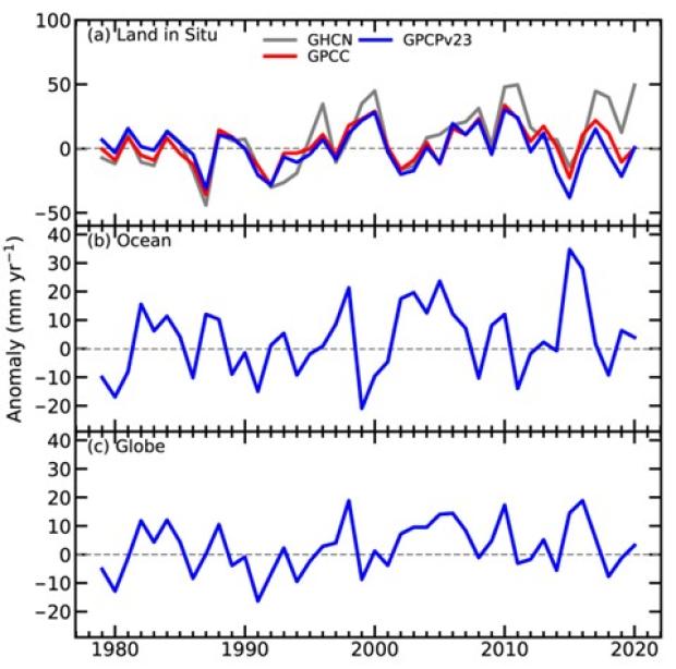
Global records of precipitation have generally not shown a clear trend except for land areas of the mid-latitudes of the northern hemisphere (Figure 5), which are increasing. In other regional areas there are likely trends observed, albeit with low confidence. For example, there was a likely reduction in southern hemisphere precipitation in the early 2000’s, and precipitation levels in tropical land areas have likely increased (Ref. 8). As shown in Figure 5, precipitation levels shown from 1900-2010 globally and at various latitudes do not show any clear trends.

Figure 5: Globally averaged precipitation anomalies (mm per year) relative to the 1981-2000 base period, over (a) land, (b) ocean, and c) the globe. Reproduced with permission from the IPCC (Ref. 8).

Ocean pH records show that globally, oceans are increasingly more acidic (lower pH). This is caused by rising levels of anthropogenic carbon dioxide (CO2) in the atmosphere, much of which gets absorbed into the ocean. Approximately 20-30% of anthropogenic CO2 emitted to the atmosphere is absorbed by the ocean. Based on a collection of records with at least a 15-year timespan, average global ocean pH has been declining by 0.017-0.027 pH units per decade (Ref. 9).

Looking forward

The 2019 IPCC Special Report, which estimates that 1.0°C of warming has already occurred globally, projects an additional 0.5°C of warming will occur between 2030 and 2052. This increase is projected to result in increases in extreme regional temperatures, increases in precipitation in some regions, and increases in drought in other regions. The temperature increase in the Arctic is projected to be two to three times the global average due to Arctic amplification, a phenomena caused by global heat flow from the equator to the poles and increased heat absorption due to reduction in snow and ice cover (Ref. 1).

Ocean heat content is projected to continue rising until at least 2040, at which point very divergent projection paths occur depending on the level of emissions. In a worst-case scenario (RCP 8.5), ocean heat content will continue rising up to 4 °C above the average through 2100. In an intermediate emissions scenario (RCP 4.5), ocean heat content will level off at about 1 degree above the average by 2040 (Ref. 3). Figure 6 shows these projected trends for the Pacific Ocean sea surface temperatures. Other ocean basins have very similar projections.

 

Figure 6: Observed and projected annual average Pacific Ocean surface temperature compared to the 1986-2000 average. The dark line shows recorded temperature values. The red band shows the range of possible temperature values under RCP 8.5, and the blue band shows the range of possible temperature values for RCP 4.5. Reproduced with permission from the IPCC (Ref. 3).

The global snow extent and duration is projected to continue reducing through 2100 as temperatures increase. Expected reductions in the northern hemisphere are up to 35% of the 1986-2005 average (Ref. 10). Projected snow thickness is more difficult to predict and changes are likely to be more regional in nature. Generally, increasing temperatures are predicted to reduce snow thickness in lower latitudes as the winter season reduces in length, while higher latitudes are predicted to increase in snow depth due to an increase in precipitation (Ref. 10).

Sea level rise is predicted to continue into the future as temperatures warm, with a sea level rise as high as 2.5 meters above 2000 levels by 2100 (Figure 7). Even with lowered emissions, sea level rise is predicted to reach at least 0.3 meters above 2000 levels by 2100 (Ref. 7). The graph below illustrates sea level rise projections with various emissions scenarios. There is increasing uncertainty on the amount of projected sea level rise further into the future, depending on many factors including the amount of Antarctic glacier melt.
 

Figure 7: Observed and projected sea level rise. Values for Change in sea level are compared to the average sea level in 2000, as illustrated in the graph. Reproduced with permission through NOAA’s free use policy – Climate.gov (Ref. 7).

There is a lot of uncertainty in projections for global precipitation levels, with various climate models showing a large variety of possible scenarios. However, mid to high latitudes do show a general projected increase in precipitation, and the equatorial ocean shows a large increase in projected precipitation (Ref. 10).

Projections of global ocean acidification are highly dependent upon which emissions pathway is followed (Figure 8). Under the worst-case scenario (RCP 8.5), ocean pH is projected to lower considerably in the near-term and continue lowering through 2100. Under the best-case scenario (RCP 2.6), ocean pH is projected to stop lowering prior to 2050 and stabilize. Regionally, oceans in high latitudes such as the Arctic Ocean are projected to have the greatest increase in ocean acidity due to their lower buffer capacity. The graph below shows climate model estimates of ocean pH levels from 1900 through 2100.

 

Figure 8: Simulated global changes in ocean surface pH from 1900-2100, compared to the1850-1900 average. RCP8.5 represents the worst-case scenario, whereas RCP2.6 represents the best-case scenario. Reproduced with permission from the IPCC – Special Report on the Ocean and Cryosphere in a Changing Climate (Ref. 9).

 

Looking Around

The trends being discussed in this indicator are global averages, and do not necessarily represent regional conditions. For example, the Arctic appears to be warming at a rate three times greater than the global average (Ref. 11). Trends in NWT climate are discussed in indicator 2.1: Trends in Observed Temperature and Precipitation in the NWT.

 

Find out more

For more information on global climate change go to the International Panel on Climate Change at http://www.ipcc.ch/index.htm

 

Technical Notes

NOAA global temperature anomaly data is derived from the Global Historical Climatology Network-Monthly (GHCN-M) data set and the International Comprehensive Ocean-Atmosphere Data Set (ICOADS), both of which are blended into a single combined land and ocean anomalies dataset. GNCN-M collects data from thousands of weather stations worldwide, and ICOADS collects surface marine data from many different observing systems worldwide.

NOAA ocean heat content data is taken from the World Ocean Database, the world’s largest collection of quality controlled publically available ocean profile data. This database represents the end result of more than twenty years of coordinated efforts to incorporate data from many different institutions, agencies, individual researchers, and data recovery initiatives.

NOAA sea level change data is acquired from the sea level group of the Commonwealth Scientific and Industrial Research Organisation (CSIRO), and the University of Hawaii Sea Level Center (UHSLC). The records are based on a weighted average of 373 global tide gauge records collected by the US National Ocean Service, UHSLC, and other partner agencies worldwide.

IPCC annual precipitation anomaly data is acquired from five data sets: the Global Historical Climatology Network, the Global Precipitation Climatology Project combined rain gauge-satellite product, the Climate Research Unit Time-Series data set, the Global Precipitation Climatology Centre data set, and a reconstructed data set by Smith et al. (Ref. 12). Each of these data sets incorporates different climate stations for each region, except the Smith et al. (Ref. 12) product which uses a statistical reconstruction over most of the global land surface area.

IPCC ocean pH data is compiled from a collection of studies from various regions of the world which used time series data from various sources such as ships, autonomous vehicles, buoys, and remote sensing. Data study periods are from as early as 1962 up to 2015.

Projections in each of the environmental variables are based on the modeling estimates of the Coupled Model Intercomparison Project (CMIP). CMIP is a collaborative framework designed to improve knowledge of the past, present and future of climate change through the use of a collection of global coupled ocean-atmosphere general circulation climate models. Results of climate projections derived through CMIP are used by the IPCC in their overall climate analysis.

 

References

Ref. 1.  IPCC. 2018: Global Warming of 1.5°C. An IPCC Special Report on the impacts of global warming of 1.5°C above pre-industrial levels and related global greenhouse gas emission pathways, in the context of strengthening the global response to the threat of climate change, sustainable development, and efforts to eradicate poverty [Masson-Delmotte, V., P. Zhai, H.-O. Pörtner, D. Roberts, J. Skea, P.R. Shukla, A. Pirani, W. Moufouma-Okia, C. Péan, R. Pidcock, S. Connors, J.B.R. Matthews, Y. Chen, X. Zhou, M.I. Gomis, E. Lonnoy, T. Maycock, M. Tignor, and T. Waterfield (eds.)]. In Press.

Ref. 2.  Lindsey, R. and Dahlman, L. 2021. National Oceanic and Atmospheric Administration – Climate.gov. “Climate Change: Global Temperature”. Available at: https://www.climate.gov/news-features/understanding-climate/climate-change-global-temperature.

Ref. 3.  Hoegh-Guldberg, O., R. Cai, E.S. Poloczanska, P.G. Brewer, S. Sundby, K. Hilmi, V.J. Fabry, and S. Jung. 2014. The Ocean. In: Climate Change 2014: Impacts, Adaptation, and Vulnerability. Part B: Regional Aspects. Contribution of Working Group II to the Fifth Assessment Report of the Intergovernmental Panel on Climate Change [Barros, V.R., C.B. Field, D.J. Dokken, M.D. Mastrandrea, K.J. Mach, T.E. Bilir, M. Chatterjee, K.L. Ebi, Y.O. Estrada, R.C. Genova, B. Girma, E.S. Kissel, A.N. Levy, S. MacCracken, P.R. Mastrandrea, and L.L.White (eds.)]. Cambridge University Press, Cambridge, United Kingdom and New York, NY, USA, pp. 1655-1731.

Ref. 4.  Dahlman, L. and Lindsey, R. 2020. National Oceanic and Atmospheric Administration – Climate.gov. “Climate Change: Ocean Heat Content”. Available at: https://www.climate.gov/news-features/understanding-climate/climate-change-ocean-heat-content.

Ref. 5.  Dahlman, L. and Lindsey, R. 2020. National Oceanic and Atmospheric Administration – Climate.gov. “Climate Change: Spring Snow Cover”. Available at: https://www.climate.gov/news-features/understanding-climate/climate-change-spring-snow-cover.

Ref. 6.  Kunkel, K. E, Robinson, D. A., Champion, S., Yin, X., Estilow, T., and Frankson, R. M. 2016. “Trends and Extremes in Northern Hemisphere Snow Characteristics”. Curr. Clim. Change Rep., DOI 10.1007/s40641-016-0036-8.

Ref. 7.  Lindsey, R.. 2021. National Oceanic and Atmospheric Administration – Climate.gov. “Climate Change: Global Sea Level”. Available at: https://www.climate.gov/news-features/understanding-climate/climate-change-global-sea-level#:~:text=Global%20mean%20sea%20level%20has,of%20seawater%20as%20it%20warms.

Ref. 8.  Hartmann, D.L., A.M.G. Klein Tank, M. Rusticucci, L.V. Alexander, S. Brönnimann, Y. Charabi, F.J. Dentener, E.J. Dlugokencky, D.R. Easterling, A. Kaplan, B.J. Soden, P.W. Thorne, M. Wild and P.M. Zhai. 2013. Observations: Atmosphere and Surface. In: Climate Change 2013: The Physical Science Basis. Contribution of Working Group I to the Fifth Assessment Report of the Intergovernmental Panel on Climate Change [Stocker, T.F., D. Qin, G.-K. Plattner, M. Tignor, S.K. Allen, J. Boschung, A. Nauels, Y. Xia, V. Bex and P.M. Midgley (eds.)]. Cambridge University Press, Cambridge, United Kingdom and New York, NY, USA.

Ref. 9.  Bindoff, N.L., W.W.L. Cheung, J.G. Kairo, J. Arístegui, V.A. Guinder, R. Hallberg, N. Hilmi, N. Jiao, M.S. Karim, L. Levin, S. O’Donoghue, S.R. Purca Cuicapusa, B. Rinkevich, T. Suga, A. Tagliabue, and P. Williamson. 2019. Changing Ocean, Marine Ecosystems, and Dependent Communities. In: IPCC Special Report on the Ocean and Cryosphere in a Changing Climate [H.-O. Pörtner, D.C. Roberts, V. Masson-Delmotte, P. Zhai, M. Tignor, E. Poloczanska, K. Mintenbeck, A. Alegría, M. Nicolai, A. Okem, J. Petzold, B. Rama, N.M. Weyer (eds.)]. In press.

Ref. 10. Collins, M., R. Knutti, J. Arblaster, J.-L. Dufresne, T. Fichefet, P. Friedlingstein, X. Gao, W.J. Gutowski, T. Johns, G. Krinner, M. Shongwe, C. Tebaldi, A.J. Weaver and M. Wehner. 2013. Long-term Climate Change: Projections, Commitments and Irreversibility. In: Climate Change 2013: The Physical Science Basis. Contribution of Working Group I to the Fifth Assessment Report of the Intergovernmental Panel on Climate Change [Stocker, T.F., D. Qin, G.-K. Plattner, M. Tignor, S.K. Allen, J. Boschung, A. Nauels, Y. Xia, V. Bex and P.M. Midgley (eds.)]. Cambridge University Press, Cambridge, United Kingdom and New York, NY, USA.

Ref. 11.Arctic Council. Arctic Climate Change Update 2021: Key Trends and Impacts – Summary for Policy-Makers. Arctic Monitoring and Assessment Programme.

Ref. 12. Smith, T. M., Arkin, P. A., Ren, L., & Shen, S. S. P. 2012. Improved Reconstruction of Global Precipitation since 1900, Journal of Atmospheric and Oceanic Technology, 29(10), 1505-1517. Available at: https://journals.ametsoc.org/view/journals/atot/29/10/jtech-d-12-00001_1.xml

 

1.3 Trends in global greenhouse gas concentrations

This indicator measures trends in greenhouse gas (GHG) concentrations in the atmosphere. GHGs are those gases which trap heat in the atmosphere. The three main human caused GHGs are carbon dioxide, methane, and nitrous oxide. Greenhouse gas concentrations refer to the amounts of those gases in the atmosphere.

 

GHGs are emitted into the atmosphere by natural processes (e.g. forest fires, thawing permafrost) and anthropogenic (e.g. burning fossil fuels, deforestation and livestock) activities. GHGs are removed from the atmosphere by chemical reactions or emission sinks (e.g. ocean, vegetation). The concentration of GHGs in the atmosphere is a reflection of the net emissions released and removed from the atmosphere.

 

Image: Industrial activity in Norman Wells, NWT. Source: ECC.

 

GHG emissions are a major contributor to atmospheric warming. GHGs prevent the loss of thermal radiation to space by absorbing thermal radiation and re-emitting thermal radiation into the atmosphere and surface of the earth. This trapping of heat by GHGs is called the greenhouse effect (Figure 1).

 

Figure 1. Greenhouse Effect. Source: Figure 2.3 of Canada’s Changing Climate Report (Ref. 1).

 

This indicator was prepared by the Government of the Northwest Territories, Department of Environment and Climate Change.

 

NWT Focus

The increase in global GHG concentrations is a major contributing factor to the noticeable changes observed in the NWT’s climate over recent decades. This increase has contributed to a variety of impacts on NWT’s environment (Ref. 2). Understanding trends in global GHG emissions can assist with climate change decision making (Ref. 2).

 

Current View: status and trend

GHG concetrations have been steadily increasing since the industrial revolution in the 18th century. GHGs remain in the atmosphere for very long periods of time, from weeks to thousands of years (Ref. 3). Although GHGs are removed from the atmosphere by chemical reactions and emission sinks, these gases are entering the atmosphere faster than they are being removed, resulting in the increase in GHGs shown in Figures 2-7.

 

Carbon Dioxide

Carbon dioxide (CO2) is the primary GHG emitted through human activities including the burning of fossil fuels. It accounts for the greatest proportion of the warming that the earth is experiencing (Figure 8, Ref. 4). The global atmospheric concentration of CO2 has increased from a pre-industrial value of approximately 280 ppm to 416 ppm in 2020 (Figure 2, 3; Ref. 5, Ref. 6). The atmospheric concentration of CO2 in 2020 far exceeds the natural range over the last 800,000 years (180 to 300 ppm) as determined from ice cores (Figure 2; Ref. 7).

Figure 2. Concentration of CO2 in the atmosphere from 800,000 Before Common Era (BCE) to 2019. Source: US Environmental Protection Agency. Ref. 7, Figure 1. Reproduction granted through the EPA free use policy.

 

Figure 3: Monthly mean carbon dioxide concentration, globally averaged over marine surface sites. Reproduced from the NOAA with permission. Ref. 6.

 

Methane

Methane (CH4) is the second most abundant human caused GHG in the atmosphere. It is 25 times more efficient than CO2 at trapping heat in the atmosphere. The global atmospheric concentration of CH4 has increased from a pre-industrial value of approximately 695 ppb to 1873 ppb in 2020 (Figure 4, 5; Ref. 8, Ref. 9). The atmospheric concentration of CH4 in 2020 far exceeds the natural range over the last 800,000 years (400 – 800 ppm) as determined from ice cores (Figure 4; Ref. 7). As evident in Figure 4, methane levelled off in the late 1990s and began rising again since 2006. It is not clear why these deviations occurred in the methane trend, however there are a number of theories. It is suggested that the mid-90's levelling off is due to the collapse of the Soviet Union and the resultant reduction in natural gas production (Ref. 10). The renewed rise since 2006 may be due to continued increases in oil and gas production, thawing wetlands, and increases in agriculture (Ref. 11).

 

Figure 4. Concentration of methane in the atmosphere from 800,000 Before Common Era (BCE) to 2019. Coloured lines represent different data sources. Source: US Environmental Protection Agency. Ref. 7, Figure 2. Reproduction granted through the EPA free use policy.

 

Figure 5. Global average monthly mean concentration of methane. Reproduced from the NOAA with permission. Ref. 9.

 

Nitrous Oxide

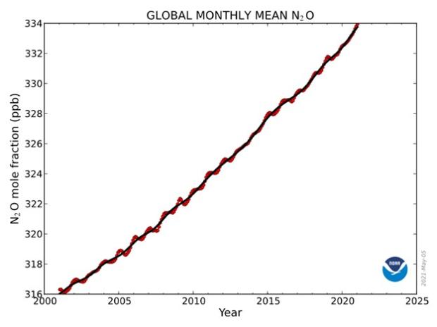
Nitrous oxide (N2O) is approximately 298 times more efficient than CO2 at trapping heat in the atmosphere. Until the present time, over the past 800,000 years, the global concentration of N2O has never exceeded 303 ppm (Figure 6; Ref. 12). Since the 1920s, levels have been increasing annually, with a concentration of 332 ppm in 2020 (Figure 7; Ref. 7, Ref. 13).

 

Figure 6. Concentration of nitrous oxide in the atmosphere from 800,000 Before Common Era (BCE) to 2015. Source: US Environmental Protection Agency. Ref. 7, Figure 3. Reproduction granted through the EPA free use policy.

 

Figure 7. Global monthly mean of nitrous oxide from 2000-2021. Reproduced from the NOAA with permission. Ref. 13.

 

Figure 8. Radiative forcing of Greenhouse Gases (GHG responsible for climate change (Ref 3) and the Annual Greenhouse Gas Index (AGGI) showing the radiative forcing, warming effect of GHGs, increased by 47% since 1990. Radiative forcing is the change in the energy balance of the Earth system due to an external change (eg GHG increases, volcanic eruption), measured in units of watts per square metre (W/m2) Ref 1. If the radiative forcing is positive the climate is warming and and if it is negative the climate is cooling. This figure shows that the total radiative forcing due to all GHGs is about 3.2 W/m2 and that CO2 is responsible for about 2.2 W/m2 of the total radiative forcing, the majority of forcing due to climate change. Figure reproduced with permission of NOAA.

 

Looking forward

The concentration of global GHGs are expected to continue increasing over the next 20 years. Increasing GHG concentrations will continue to warm the earth’s atmosphere, causing an increase in sea levels and ocean temperature, a decrease in freshwater availability (Ref. 14), an increase in extreme weather events, and an increase in permafrost thaw. All of these physical changes will lead to impacts on ecosystems, communities, and the health, well-being and livelihoods of humans.

One of the best examples of a cascading effect of these changes is the impact of massive permafrost thaw in Arctic regions. Permafrost acts as a large store of carbon, and as it thaws it releases this carbon as GHGs into the atmosphere. The amount of carbon released as permafrost thaws is estimated to reach 23-174 petagram[1] (Pg) of carbon under the high-emissions scenario (RCP 8.5). While this is a large range of potential outcomes, even the low end of this range is substantially greater than the annual amount emitted from fossil fuel use during 2009-2018 (9.5 Pg; Ref. 15). Such a large contribution of GHGs to the atmosphere will drive even further warming of the planet, resulting in a positive feedback loop.

The Paris Agreement, which was adopted by 196 parties, aims to reduce GHG emissions and limit global warming to below 2°C (preferably to 1.5°C). However, there are numerous challenges in reaching this goal. For example, there are financial, technical, and social challenges that exist in vulnerable countries which may cause challenges in implementing changes to reduce emissions. Additionally, technologies such as carbon removal are still in the early research stages or don’t exist at any meaningful scale as of yet. Lastly, the political will to set stronger policy changes to curtail emissions more significantly may not exist in many countries. Current pledges (Ref 16) could limit warming to 2 ° C, unfortunately, under existing policies the median estimates of 2100 warming are modeled to be approximately 2.6 °C, with a range of 2 °C to 3.7 °C. Current polices may not meet the Paris Agreement target of 2° C.

 

Find out more

For more information on global climate change go to the Intergovernmental Panel on Climate Change at https://www.ipcc.ch/.

 

References

Ref. 1.  Environment and Climate Change Canada. 2019. Canada’s Changing Climate Report. Available at: https://changingclimate.ca/CCCR2019/.

Ref. 2.  GNWT. 2018. 2030 NWT Climate Change Strategic Framework. Available at: https://www.ecc.gov.nt.ca/sites/enr/files/resources/128-climate_change_strategic_framework_web.pdf.

Ref. 3.  United States Environmental Protection Agency. 2021. Climate Change Indicators: Greenhouse Gases. Available at: https://www.epa.gov/climate-indicators/greenhouse-gases.

Ref 4. National Oceanic and Atmospheric Oceanic Index. 2021. THE NOAA ANNUAL GREENHOUSE GAS INDEX (AGGI). NOAA Global Monitoring Laboratory. Earth System Research Laboratories. https://gml.noaa.gov/aggi/aggi.html.

Ref. 5.  United States Environmental Protection Agency. 2021. Global atmospheric carbon dioxide concentration time series data. Available at: https://www.epa.gov/sites/production/files/2021-03/ghg-concentrations_fig-1.csv.

Ref. 6.  National Oceanic and Atmospheric Administration – Global Monitoring Laboratory. 2021. Trends in Atmospheric Carbon Dioxide. Available at: https://gml.noaa.gov/ccgg/trends/global.html.

Ref. 7.  United States Environmental Protection Agency. 2021. Climate Change Indicators: Atmospheric Concentrations of Greenhouse Gases. Available at: https://www.epa.gov/climate-indicators/climate-change-indicators-atmospheric-concentrations-greenhouse-gases.

Ref. 8.  United States Environmental Protection Agency. 2021. Global atmospheric methane concentration time series data. Available at: https://www.epa.gov/sites/production/files/2021-03/ghg-concentrations_fig-2.csv.

Ref. 9.  National Oceanic and Atmospheric Administration – Global Monitoring Laboratory. 2021. Trends in Atmospheric Methane. Available at: https://gml.noaa.gov/ccgg/trends_ch4/.

Ref. 10.Johnson, S.K. 2016. Why did methane stop increasing, then start again? ArsTechnica - Science. Available at: https://arstechnica.com/science/2016/03/why-did-methane-stop-increasing-then-start-again/.

Ref. 11.NASA. 2018. NASA-led Study Solves a Methane Puzzle. Available at: https://www.nasa.gov/feature/jpl/nasa-led-study-solves-a-methane-puzzle.

Ref. 12. United States Environmental Protection Agency. 2021. Global atmospheric nitrous oxide concentration time series data. Available at: https://www.epa.gov/sites/production/files/2021-03/ghg-concentrations_fig-3.csv.

Ref. 13. National Oceanic and Atmospheric Administration – Global Monitoring Laboratory. 2021. Trends in Atmospheric Nitrous Oxide. Available at: https://gml.noaa.gov/ccgg/trends_n2o/.

Ref. 14.Schewe, J., Heinke J., Gerten D., Haddeland, I., Arnell, N.W., Clark, D.B., Dankers, R., Eisner, S., Fekete, B.M., Colon-Gonzalez, F.J., Goslin, S.N., Kim, H., Liu, X., Masaki, Y., Portmann, F.T., Satoh, Y., Stacke, T., Tang, Q., Wada, Y., Wisser, D., Albrecht, T., Frieler, K., Piontek, F., Warszawski, L., and Kabat, P. 2013. Multimodal assessment of water scarcity under climate change. Proceedings of the National Academy of Sciences, v.111(9), pp. 3245-3250.

Ref. 15. Nature Geoscience. 2020. When permafrost thaws. Nat. Geosci. 13, 765. Available at: https://doi.org/10.1038/s41561-020-00668-y.

Ref. 16.Hausfather, Z., and Moore, F.C. 2022. Commitments could limit warming to below 2°C. Nature, v. 604, pp. 247-248.

 

 

1.4 Global Climate Linkages (Teleconnections)

 

This indicator tracks a number of global climate teleconnections, or the linkages in climate between geographically separated regions (Ref. 1), including the Arctic Oscillation (AO), North Atlantic Oscillation (NAO), El Niño-Southern Oscillation (ENSO), Pacific Decadal Oscillation (PDO), and the Scandinavian Pattern (SP).

Image: Illustration of global oscillations. Used with permission of the Woods Hole Oceanographic Institution.

This indicator was prepared by the Government of the Northwest Territories, Department of Environment and Climate Change.

 

NWT Focus

While most teleconnections do not show apparent long-term trends, they are important as they explain much of the variability in climate within a timescale of weeks to decades (Ref. 2). In general, patterns of atmospheric teleconnections alter between two different phases. The best known are the El Niño (warm, positive) vs La Niña (cold, negative) phases of the ENSO teleconnection. The change from one phase to another is generally driven by pressure changes in the atmosphere and temperature changes in the ocean. Each of the different atmospheric teleconnections described below takes place over a wide-reaching geographical area. While each of these teleconnections is distinct, they affect one another and so teleconnections occurring in one global area tend to influence teleconnections in other areas.

Many different atmospheric oscillations around the globe can influence the conditions in the NWT. Discussion of the main teleconnections is very important because their effects will combine with a changing climate and influence the NWT’s weather in particular years and decades. For example, very late openings of winter roads in the NWT have been associated with strong El Niño phase events (Ref. 3); warming in the central Pacific due to El Niño contributes to cooler summer Arctic temperatures (Ref. 4); winter stream flows have been found to be higher during the warm phase of the PDO (Ref. 5); extremely large NWT forest fire years have been associated with the negative phase of the summertime AO (Ref. 6); variations in the rate of Arctic sea ice loss have been associated with the PDO (Ref. 7); a newly identified high latitude anti-cyclonic atmospheric circulation connected to the SP has been shown to boost heatwave frequencies and increase rates of wildfire events in the Arctic (Ref. 8); and tree-ring reconstruction of streamflow in the Snare River Basin (the watershed that supplies Yellowknife with the majority of its hydroelectricity) has been shown to be well correlated with the NAO (Ref. 9). These atmospheric oscillations can also minimize the effects of a warming climate in particular years: a cool spring experienced in the NWT in 2021 is associated with a La Niña event in the Pacific Ocean (see El Niño/Southern Oscillation section below).

Teleconnections are important in explaining decadal and year to year weather variability in the NWT in addition to the effects of a change climate.

Some patterns of teleconnections themselves are changing due to climate change (see El Niño/Southern Oscillation). One of the most significant impacts in the NWT may be when teleconnections amplify the effects of climate change. Wan et al. (Ref. 10) have found that up to 0.5°C of the observed warming trend in Canada may be due to teleconnections.

It should be noted that while clear connections have been shown between weather and climate in the NWT and global teleconnections, there is a great deal of uncertainty in the relative amount of influence each of the various teleconnections has in the NWT. Exactly what types of influence each of the teleconnections might have, and how much of the variation in NWT weather and climate is independent of global teleconnections are areas of current research.

 

Current View: status and trend

Arctic Oscillation

The Arctic Oscillation (AO) covers all areas north of 55°N latitude, so is perhaps the most relevant to the NWT. The AO is an atmospheric oscillation involving changes in the wind patterns surrounding the cold, low pressure air that covers the Arctic, known as the polar vortex. During the positive phase of the AO, the pressure difference between the polar vortex and the atmosphere in more southerly latitudes remains distinct, driving a strong counter-clockwise wind at the edge of the polar vortex, known as the polar jet stream, which circles the globe, preventing any mixing of the polar vortex and surrounding atmosphere in the south. However, during the negative phase of the AO, the pressure differences between the polar vortex and the surrounding atmosphere become less distinct, causing the polar jet stream to weaken and become more turbulent. This turbulence allows much more mixing of the cold polar vortex air with the southerly warmer air (Ref. 11, Ref. 12, Ref. 13), resulting in highly chaotic temperature patterns in which cold periods will occur in southerly regions and warm spells can occur high in the Arctic (Ref. 11).

As shown in Figure 1, the AO has a strong influence on wintertime weather in the Northern Hemisphere. In the positive phase cold air stays north and in the negative phase cold arctic air reaches much of North America due to the wavy pattern of the jet stream.

The AO can oscillate between phases from anywhere between days and months at a time (Ref. 12), although its longer-term pattern appears unpredictable. The AO is noted to have been strongly positive in the early 1990’s compared to the previous 40 years, and became closer to negative thereafter (Ref. 14; Figure 1), resulting in milder temperatures in the Arctic. The positive phase of the Arctic Oscillation results in approximately 5°C warmer temperatures in southern Canada and the US than the negative phase, and colder temperatures in northern regions such as the NWT (Ref. 15).

The AO index is used to track the AO phase shifts. Figure 2 shows the seasonal mean AO index for the cold season (January, February, March). The cold season is relevant because it is during the winter months that the AO has the greatest variability (Ref. 16).

 

Figure 1: The two phases of the Arctic Oscillation. (AO) The AO index is a measure of the pressure difference between the polar vortex (blue zone) and the surrounding atmosphere, (purple zone). In the negative phase, cold air spills south and warm air moves north due to the wavy pattern in the jet stream. In the positive phase, cold air stays north. Source: National Oceanic and Atmospheric Administration (Ref. 17). Permission granted through NOAA’s free use policy.

Figure 2: The standardized seasonal mean Arctic Oscillation index during the cold season (average of January, February, March) from 1950-2021, shown with the blue line. The black line is the five-year running mean of the index. Reproduced from NOAA National Weather Service Climate Prediction Center (Ref. 16). Reproduced with permission through NOAA’s free use policy.

The AO is strongly correlated with the North Atlantic Oscillation, which is described below.

 

North Atlantic Oscillation

Closely related to the AO is the North Atlantic Oscillation (NAO). In fact, due to their proximity, the NAO is highly correlated with the AO, and some atmospheric scientists debate that they are one and the same (Ref. 18). The NAO is an atmospheric oscillation occurring between the high north Atlantic Ocean, centered over Iceland, and the central Atlantic Ocean, centered over the Azores. In its positive phase, atmospheric pressure is lower than average over Iceland, and higher than average over the Azores. In its negative phase, the opposite occurs. These phase changes are caused by the back and forth movement of air masses over the north Atlantic Ocean. It can perhaps best be imagined as similar to a tub of water sloshing back and forth.

Changes in these phases have climatic effects over a wide-ranging area around the north Atlantic, including eastern North America and western Europe (Ref. 19, Ref. 20). The positive phase of the NAO is associated with above-average temperatures in eastern North America and northern Europe and below-average temperatures in Greenland and sometimes southern Europe and the Middle East. It has also been associated with above-average precipitation in northern Europe and below-average precipitation in central and southern Europe (Ref. 19).

The NAO index is used to track the NAO. This index is a measure of the atmospheric pressure difference between Iceland and the Azores. Figure 3 shows the seasonal mean NAO index for the cold winter (January, February, March). The wintertime NAO displays significant variability between 1950 and 2021 (Figure 3). The NAO exhibits considerable variability on time scales from seasons to decades (Ref. 21).

Because the northern reach of the NAO is directly adjacent to the AO, it is strongly influenced by the AO. In fact, these two systems are so strongly linked that many meteorologists consider the NAO to be a regional subset of the AO (Ref. 20). Similarities can be seen by comparing the AO graph (Figure 2) and the NAO graph (Figure 3).

Figure 3: The standardized seasonal mean North Atlantic Oscillation index during the cold season (average of January, February, March) from 1950-2021, shown with the blue line. The black line is the five-year running mean of the index. Reproduced from NOAA National Weather Service Climate Prediction Center (Ref. 21). Reproduced with permission through NOAA’s free use policy.

 

El Niño/Southern Oscillation

The El Niño/Southern Oscillation (ENSO) is perhaps the most well-known atmospheric oscillation system. ENSO takes place over the equatorial Pacific Ocean. Under normal circumstances, atmospheric pressure is lower in the western equatorial Pacific than the eastern equatorial Pacific, causing a westward wind which blows the surface waters of the equatorial Pacific west towards Australia. In the eastern Pacific, near the western coast of South America, as these warm surface waters are blown west they are replaced by deeper water upwelling to the surface, which is cooler and nutrient-dense. Thus, a circulation of water occurs in the equatorial Pacific which moves warm surface water west and cooler deep water up to the surface in the east. This cycle is further reinforced by a positive feedback loop in which warmer western surface water causes a warmer, more buoyant atmosphere which rises and further enhances the winds blowing from the east, thereby continuing to drive warm surface water west. During an El Niño event, however, the atmospheric pressure differential between the eastern and western Pacific weakens, reducing the western winds, and thereby slowing the ocean circulation as well. The result is a cooler western Pacific with less warm surface water, and a warmer eastern Pacific where warm surface waters can build up (Ref. 22). During a La Niña event, the opposite occurs – the atmospheric pressure differential between the eastern and western Pacific is stronger than normal, causing strengthened western winds. The result is even more warm water pushed towards Australia than normal, and greater upwelling from deep, cool water in the eastern Pacific (Ref. 23).

The impact of the ENSO is felt most strongly in Australia and equatorial South America. During La Niña (positive phase), warm water is drawn to the western Pacific and causes increased precipitation in Australia and much less rain in South America, while during El Niño (negative phase) conditions, the opposite it true – warm waters move to the eastern Pacific, causing abundant rainfall in South America and drought conditions in Australia (Ref. 21). However, the ENSO is a strong driver of change in many other areas of the world as well. During El Niño conditions, the warm eastern Pacific waters cause warm, moist air to form in a process called latent heating. This warm air rises to the upper atmosphere, where it spreads poleward through Hadley circulation[1]. This added heat moving poleward through the atmosphere causes changes in temperature and precipitation in many areas worldwide (Ref. 22). North America, for example, is strongly affected by ENSO. During El Niño, areas in northwestern North America, including the NWT, are warmer and dryer than normal. During La Niña, the opposite is true – northwestern North America tends to be cooler and wetter than normal. Figure 4 shows the effect of the two phases of ENSO on North America.

[1] The Hadley circulation or cell is a pattern of atmospheric circulation from the equator to approximately latitude 25° north and south of the equator (Ref. 22). Warm air rises at the equator (low pressure at surface), moves poleward at altitude, and sinks in the subtropics (high pressure at surface) returning towards the equator at the surface through the trade winds. The net result of the Hadley circulation is to transport energy poleward, compensating for the unequal distribution of solar energy.

 

Figure 4: The effect of the ENSO cycle on North America. a) Effects from El Niño. b) Effects from La Niña. Reproduced with permission from the NOAA (Ref. 23), through their free use policy.

There are a number of indexes used to track ENSO. A common measure is the Southern Oscillation Index (SOI), which measures the difference in atmospheric pressure at sea level between Darwin, Australia and Tahiti (Ref. 26). Another index which is the standard for the National Oceanographic and Atmospheric Administration NOAA is the Oceanic Niño Index (ONI). The ONI tracks the running 3-month average sea surface temperature in the east-central tropical Pacific between 120°-170°W. This value is then compared to a 30-year average, and the difference is the ONI value. An ONI value of +0.5 or greater indicates El Niño conditions, and an ONI value of -0.5 or less indicates La Niña conditions, given consistent atmospheric features and a forecast of anomalous conditions persisting for 3 consecutive months (Ref. 27). Figure 5 shows a historical record of the ONI since 1950, with clearly identifiable periods of El Niño and La Niña conditions. The period of the ENSO cycle averages four years, although it has historically been quite variable with a period of anywhere from two to seven years (Ref. 26).

The strength of El Niño events has increased since the 1970s (Figure 6). Wang et al (Ref. 28) suggest that this increase in extreme El Niño events is due to climate change. Figure 6 shows that the location of strong El Niño events has shifted from the Eastern Pacific prior to 1978, westward to include the Central Pacific and Basin Wide (central and eastern Pacific).

It should be noted that while the strong link between atmospheric pressure and ocean temperatures is well understood in the ENSO cycle, there is still little understanding of what mechanism initiates the oscillation from one phase to another (Ref. 22).

Figure 5: The Oceanic Niño index from 1950 to May 2021. The ONI tracks the running 3-month average sea surface temperatures in the east-central tropical Pacific between 120°W and 170°W. The ONI index value is the difference between the current 3-month average sea surface temperature and a 30-year average. The red and blue lines indicate the threshold for El Nino conditions (greater than +0.5; above the red line) and La Nino conditions (less than -0.5; below the blue line). Reproduced with permission from the NOAA (Ref. 27), through their free use policy.

Figure 6: Since the late 1970s the strength of El Niño events has increased as can be seen in the high ONI index values approaching 2.0. Prior to the 1970s, strong El Niño events were in the Eastern Pacific (EP). Since the 1970s, strong El Niño have been located in the Central Pacific (CP) of basin wide (Eastern and Central). The dashed line indicates El Niño conditions. Source: Wang et al. (Ref. 28). Reproduced with permission from the Proceedings of the National Academy of Sciences of the United States of America.

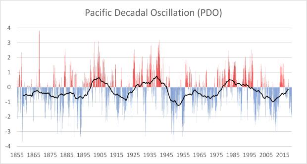
Pacific Decadal Oscillation

The Pacific Decadal Oscillation (PDO) takes place over the north Pacific Ocean and oscillates between two phases known as the warm phase and cool phase. During the warm (or positive) phase, the PDO consists of warmer than average waters off the west coast of North America, and colder than average waters further out in the central north Pacific Ocean. During the cool (or negative) phase, the opposite is true (Ref. 29).

There is a wide range of factors known to influence the PDO. The main ones include:

1. The Aleutian Low (AL). The AL is an area of consistently low atmospheric pressure centered near the Aleutian Islands. As air from higher-pressure surrounding areas flows in, it circles the AL, much like water draining out of a sink. Because the AL is located in the northern hemisphere, the air circles in a counter-clockwise direction. This means that west of the AL, winds are blowing down from the northeast, and east of the AL, winds are blowing up from the southwest. During a positive PDO phase, the AL has a lower atmospheric pressure than average, and the high pressure differential between the AL and surrounding air creates strong winds. In the west, the strong northerly winds blow cold Arctic surface waters down into the central Pacific. In the east, near the west coast of North America, the strong southerly winds blow warm surface waters up the coast from warmer, lower latitude seas. During a negative PDO phase, the AL has higher atmospheric pressure than average, and therefore the winds are weaker and are far less effective at moving the surface water (Ref. 29).

2. ENSO. The ENSO cycle, which is another oscillation occurring in the equatorial Pacific Ocean and explained in more detail above, has a strong influence on the PDO since they are geographically adjacent to one another. ENSO’s El Niño (negative) phase tends to cause a stronger than average AL, while the La Nina (positive) phase tends to weaken the AL (Ref. 29).

3. Deep ocean memory. Sea surface temperature anomalies can work their way to depth over time, warming (or cooling) the deeper ocean layers as well. Then, when things change on the surface, the temperature of the deeper ocean layers is often preserved and acts to revert sea surface temperatures back to their previous state. This phenomenon is known as “re-emergence” and it allows for greater stability and endurance of different phases of the PDO (Ref. 29).

4. The Kuroshio Current. The Kuroshio Current is a large ocean current originating in the East China Sea and extending out towards the central Pacific. This is a warm current and so transports heat into the central Pacific. However, this current is fairly turbulent and can alter its location and strength over a period of decades (Ref. 30). This means that the amount and location of heat entering the western side of the north Pacific Ocean from the Kuroshio Current varies considerably over decades and affects the PDO (Ref. 29).

Impacts of the PDO can be felt near the coast in both eastern Asia and western North America, primarily through changes in the amount of rainfall (Ref. 30, Ref. 31, Ref. 32, Ref. 33). However, it should be noted that the PDO may not cause far-reaching effects. For example, changes in rainfall across western North America has been found to be more closely associated with the ENSO than with the PDO (Ref. 31).

Because there are so many factors that influence the PDO, its period is far more variable than other oscillations such as ENSO. However, a number of studies have used a paleoproxy climate indicator such as tree rings to extend the record and determine a longer-term trend for the PDO (Ref. 31, Ref. 32, Ref. 33, Ref. 34). MacDonald and Case (2005) used their extended record to identify a 50-70 year periodicity in the PDO for the past 200 years, but with much less predictability prior to 200 years ago. They also identified a prolonged period of negative PDO from 993 AD to 1300 AD (Ref. 34).

Figure 7 shows positive and negative phases of the PDO since 1854. This graph is based on sea surface temperature measurements derived from the International Comprehensive Ocean-Atmosphere Dataset, which is a compilation of surface marine data from many different observing systems over the past three centuries (Ref. 36).

Figure 7: The monthly Pacific Decadal Oscillation Index from 1854-2021. The PDO Index is determined as by the sea surface temperature anomaly compared to the 1971-2000 average. The black line represents the 10 year moving average. Data derived from NOAA (Ref. 36). Reproduced with permission through NOAA’s free use policy.

The Scandinavian Pattern

The Scandinavian Pattern (SP) is an atmospheric oscillation occurring between western Norway and the northeastern Atlantic Ocean near Greenland (Ref. 37). The positive phase of the SP is associated with anticyclones over Scandinavia and western Russia, below-average temperatures across central Russia and western Europe, above-average precipitation across central and southern Europe, and below-average precipitation across Scandinavia (Ref. 38).

Yasunari et al. (Ref. 8) has identified a new atmospheric pattern called the circum-Arctic wave (CAW) which is associated with the negative phase of the SP. The CAW is a clockwise circulation pattern which produces anomalously hot and dry conditions across the north, resulting in increased forest fires. Interestingly, the researchers found that the CAW has only been significant since 2003.

 

Looking forward

The various global atmospheric oscillations are generally highly variable and chaotic in nature. Therefore, it is difficult to provide any specific predictions on how climate change may affect these oscillations. Climate models appear to project some general atmospheric changes, such as a poleward shift in the mid-latitude jets and a widening and weakening of Hadley circulation in the northern hemisphere (Ref. 39). There have been attempts to predict changes in specific atmospheric oscillations. For example, Hamouda et al. (Ref. 39) use climate model simulations to predict a decoupling of the AO and NAO under a strong warming scenario. Wang et al. (Ref. 28) use historical ENSO data to predict increased extreme El Niño events in the future.

Even extremely short-term predictions are difficult. For example, a consortium of researchers have attempted to use the Tropical Pacific Observing System (TPOS), which is a network of Pacific climate observing stations, to forecast immediate short-term changes in the ENSO cycle. These predictions have generally failed, such as in 2014, when many researchers predicted an extremely strong El Niño which failed to materialize. This consortium is now focused on improving TPOS to provide more robust data and allow a deeper dive into the problem of forecasting the ENSO (Ref. 41).

 

Technical Notes

The AO Index is determined by projecting the AO loading pattern to the daily anomaly 1000 millibar height field over 20°N-90°N latitude. The AO loading pattern is the first mode of empirical orthogonal function analysis using monthly mean 1000 millibar height anomaly data from 1979 to 2000 over 20°N-90°N latitude (Ref. 11).

The NAO index is determined by projecting the NAO loading pattern to the daily anomaly 500 millibar height field over 0-90°N latitude. The NAO loading pattern is the first mode of a rotated empirical orthogonal function analysis using monthly mean 500 millibar height anomaly data from 1950 to 2000 over 0-90°N latitude (Ref. 19).

The PDO Index shown in the corresponding graph is the National Centers for Environmental Information (NCEI) PDO Index. This index is based on the National Oceanic and Atmospheric Administration’s (NOAA) extended reconstruction of sea surface temperatures (ERSST), and is constructed by regressing the ERSST anomalies against the Mantua PDO Index for their overlap period, to compute a PDO regression map for the North Pacific ERSST anomalies. The ERSST anomalies are then projected onto that map to compute the NCEI Index. The NCEI PDO index closely follows the Mantua PDO Index (Ref. 40). The ERSST is derived from the International Comprehensive Ocean-Atmosphere Dataset (ICOADS) (Ref. 42).

The SOI shown in the corresponding graph is based on a measure of the sea level atmospheric pressure difference between Darwin, Australia and Tahiti. It is calculated as the difference in the standardized pressure between Tahiti and Darwin, divided by the monthly standard deviation (Ref. 43).

 

References

Ref. 1. Nigam, S, and S. Baxter. 2014 Teleconnections in Encyclopedia of Atmospheric Sciences. 2nd Ed. Elsevier pp. 90-109.

Ref. 2.  Goodrich. G. 2016. Atmospheric Teleconnections. Oxford Bibliographies Online. DOI: 10.1093/OBO/9780199874002-0147

Ref. 3.  Knowland, K.E., Gyakum, J.R., & Lin, C.A. 2010. A study of the meteorological conditions associated with anomalously early and late openings of a Northwest Territories winter road. Arctic, 63(2), 227–239.

Ref. 4. Hu, C., Yang, S., Wu, Q., Li, Z., Chen, J., Deng, K., Zhang, T., and Zhang, C. 2016. Shifting El Niño inhibits summer Arctic warming and Arctic sea-ice melting over the Canada Basin. Nature Communications, 7:11721.

Ref. 5.  Khaliq, M.N. and P. Gachon. 2010. Pacific Decadal Oscillation Climate Variability and Temporal Pattern of Winter Flows in Northwestern North America. Journal of Hydrometeorology. 11: 917-933.

Ref. 6.  Fauria, M.M. and E.A. Johnson. 2008. Climate and wildfires in the North American boreal forest. Phil. Trans. R. Soc. B. 363: 2317-2329.

Ref. 7.  Bonan D B and Blanchard-Wrigglesworth E. 2020. Nonstationary teleconnection between the Pacific Ocean and Arctic sea ice Geophys. Res. Lett. 47 e2019GL085666.

Ref. 8.  Yasunari, T. J., Nakamura, N., Kim, K. -M., Choi, N., Lee, M. –I., Yachibana, Y., and da Silva, A. M. 2021. Relationship between circum-Arctic atmospheric wave patterns and large-scale wildfires in boreal summer. Environmental Research Letters, v. 16(6).

Ref. 9. Martin, J.P. and Pisaric, M.F. 2017. Tree-ring reconstruction of streamflow in the Snare River Basin, Northwest Territories, Canada. American Geophysical Union, Fall Meeting 2017, abstract #PP31A-1247.

Ref. 10. Wan. H. Z. Zhang. F. Zwiers. 2019. Human Influence on Canadian Temperatures. Climate Dynamics. 52-479-494.

Ref. 11. National Oceanic and Atmospheric Administration. 2021. Arctic Oscillation (AO). May 2021 version. Available at: https://www.ncdc.noaa.gov/teleconnections/ao/.

Ref. 12. National Snow & Ice Data Center. 2020. What is the Arctic Oscillation?. October 2020 version. Available at: https://nsidc.org/cryosphere/icelights/2012/02/arctic-oscillation-winter-storms-and-sea-ice.

Ref. 13. National Oceanic and Atmospheric Administration. 2014. How is the polar vortex related to the Arctic Oscillation?. January 2014 version. .Available at: https://www.climate.gov/news-features/event-tracker/how-polar-vortex-related-arctic-oscillation.

Ref. 14. National Oceanic and Atmospheric Administration – Arctic Change Indicators Website.2021. “Climate Indicators – Arctic Oscillation”. Available at: https://www.pmel.noaa.gov/arctic-zone/detect/climate-ao.shtml.

Ref. 15. Thompson, D. W. and J. M. Wallace. 2001. Regional Climate Impacts of the Northern Hemisphere Annual Mode. Science. 293(5527), 85-89.

Ref. 16. National Oceanic and Atmospheric Administration – National Weather Service Climate Prediction Center. 2021. Arctic Oscillation (AO). Available at: https://www.cpc.ncep.noaa.gov/products/precip/CWlink/daily_ao_index/ao.shtml.

Ref. 17. National Climatic Data Center, National Oceanic and Atmospheric Administration .2010. State of the climate in 2010 – Highlights. Available at http://www1.ncdc.noaa.gov/pub/data/cmb/bams-sotc/2010/bams-sotc-2010-brochure-hi-rez.pdf.

Ref. 18.National Oceanic and Atmospheric Administration – climate.gov. 2021. Climate Variability: North Atlantic Oscillation. Available at: https://www.climate.gov/news-features/understanding-climate/climate-vari....

Ref. 19. National Oceanic and Atmospheric Administration. 2021. North Atlantic Oscillation (NAO). Available at: https://www.ncdc.noaa.gov/teleconnections/nao/.

Ref. 20. Lindsey, R. 2011. Long Distance Relationships: the Arctic and North Atlantic Oscillations. March 2011 version, National Oceanic and Atmospheric Administration. Available at: https://www.climate.gov/news-features/understanding-climate/long-distance-relationships-arctic-and-north-atlantic.

Ref. 21. National Oceanic and Atmospheric Administration – National Weather Service Climate Prediction Center. North American Oscillation (NAO). Available at: https://www.cpc.ncep.noaa.gov/products/precip/CWlink/pna/nao.shtml.

Ref. 22. National Oceanic and Atmospheric Administration. 2021. El Niño/Southern Oscillation (ENSO) Technical Discussion. Available at: https://www.ncdc.noaa.gov/teleconnections/enso/enso-tech.php.

Ref. 23. National Oceanic and Atmospheric Administration – National Ocean Service.2021. What are El Niño and La Niña?. Available at: https://oceanservice.noaa.gov/facts/ninonina.html.

Ref. 24. Barnston, A. 2014. How ENSO leads to a cascade of global impacts. May 2014 version. National Oceanic and Atmospheric Administration – Climate.gov. Available at: https://www.climate.gov/news-features/blogs/enso/how-enso-leads-cascade-global-impacts.

Ref. 25. James, I.N. 2002. Hadley Circulation. In (J.R. Holton. Ed) Encyclopedia of Atmospheric Sciences. Elsevier Science. 919-924.

Ref. 26. National Oceanic and Atmospheric Administration – National Weather Service Climate Prediction Center. 2021. The Southern Oscillation Index (SOI). Available at: https://www.cpc.ncep.noaa.gov/products/analysis_monitoring/ensocycle/soi.shtml.

Ref. 27. National Oceanic and Atmospheric Administration – Climate Prediction Center. 2021. “ENSO: Recent Evolution, Current Status and Predictions”. PowerPoint presentation. Accessed June 2021. Available at: https://www.cpc.ncep.noaa.gov/products/analysis_monitoring/lanina/enso_evolution-status-fcsts-web.pdf.

Ref. 28. Wang, B., Luo, X., Yang, Y.-M., Cane, M. A., Cai, W., Yeh, S.-W., and Liu, J. 2019. Historical change of El Nino properties sheds light on future changes of extreme El Nino. Proceedings of the National Academy of Sciences of the United States of America, v. 116, Issue 45, pp. 22512-22517.

Ref. 29. Di Liberto, T. 2016. Going out for ice cream: a first date with the Pacific Decadal Oscillation. August 2016.version, National Oceanic and Atmospheric Administration – Climate.gov. Available at: https://www.climate.gov/news-features/blogs/enso/going-out-ice-cream-first-date-pacific-decadal-oscillation.

Ref. 30. Nagai, T. 2019. The Kuroshio Current: Artery of Life, Eos, 100, https://eos.org/editors-vox/the-kuroshio-current-artery-of-life. Published on 27 August 2019.

Ref. 31. Biondi, F., Gershunov, A., and Cayan, D. R. 2001. North Pacific Decal Climate Variability since 1661. Journal of Climate, v. 14, Issue 1, pp. 5-10.

Ref. 32. Wang, W.-C., Gong, W., and Hao, Z. 2006. A Pacific Decadal Oscillation record since 1470 AD reconstructed from proxy data of summer rainfall over eastern China. Geophysical Research Letters, 33(3): L03702. Available at https://agupubs.onlinelibrary.wiley.com/doi/pdf/10.1029/2005GL024804

Ref. 33. D’Arrigo, R. and Wilson, R. 2006. On the Asian expression of the PDO. International Journal of Climatology, 26(12): 1607-1617.

Ref. 34. MacDonald, G. M. and Case, R. A. 2005. Variations in the Pacific Decadal Oscillation over the past millennium. Geophysical Research Letters, 32(8): L08703 Available at https://agupubs.onlinelibrary.wiley.com/doi/pdfdirect/10.1029/2005GL022478

Ref. 35. National Oceanic and Atmospheric Administration - International Comprehensive Ocean. 2021.Atmosphere Data Set. Available at: https://icoads.noaa.gov/.

Ref. 36. National Oceanographic and Atmospheric Administration, National Centers for Environmental Information. 2021. Pacific Decadal Oscillation (PDO). Accessed July 2, 2021 Available at https://www.ncdc.noaa.gov/teleconnections/pdo/

Ref. 37. Majeed, H. and Moore, G. W. K. 2018. Influence of the Scandinavian climate pattern on the UK asthma mortality: a time series and geospatial study. Public Health, 8(4).

Ref. 38. National Oceanic and Atmospheric Administration – National Weather Service Climate Prediction Center. 2021. Scandinavia (SCAND). Available at: https://www.cpc.ncep.noaa.gov/data/teledoc/scand.shtml.

Ref. 39. Collins, M., R. Knutti, J. Arblaster, J.-L. Dufresne, T. Fichefet, P. Friedlingstein, X. Gao, W.J. Gutowski, T. Johns, G. Krinner, M. Shongwe, C. Tebaldi, A.J. Weaver and M. Wehner. 2013: Long-term Climate Change: Projections, Commitments and Irreversibility. In: Climate Change 2013: The Physical Science Basis. Contribution of Working Group I to the Fifth Assessment Report of the Intergovernmental Panel on Climate Change [Stocker, T.F., D. Qin, G.-K. Plattner, M. Tignor, S.K. Allen, J. Boschung, A. Nauels, Y. Xia, V. Bex and P.M. Midgley (eds.)]. Cambridge University Press, Cambridge, United Kingdom and New York, NY, USA.

Ref. 40. Hamouda, M. E., Pasquero, C., and Tziperman, E. 2021. Decoupling of the Arctic Oscillation and North Atlantic Oscillation in a warmer climate. Nature Climate Change, 11: 137-142.

Ref. 41. Smith, N., Kessler, W. S., Hill, K. and Carlson, D. 2015. Progress in Observing and Predicting ENSO. World Meteorological Organization Bulletin, 64(1).

Ref. 42. National Oceanic and Atmospheric Administration. 2021. Extended Reconstructed Sea Surface Temperature (ERSST) v5. Available at: https://www.ncdc.noaa.gov/data-access/marineocean-data/extended-reconstructed-sea-surface-temperature-ersst-v5.

Ref. 43. National Oceanic and Atmospheric Administration. 2021. Southern Oscillation Index (SOI). Available at: https://www.ncdc.noaa.gov/teleconnections/enso/indicators/soi/.